4.2. 동적 시간 워핑 (DTW)

Dynamic Time Warping

두 음악/오디오 시퀀스를 최적의 방법으로 시간에 따라 정렬할 수 있는 동적 시간 워핑 (dynamic time warping, DTW)에 대해 설명한다.

이 글은 FMP(Fundamentals of Music Processing) Notebooks을 참고로 합니다.

import numpy as np
import pandas as pd
import matplotlib.pyplot as plt
import librosa
import librosa.display
import IPython.display as ipd
from IPython.display import Image

import scipy.spatial
from utils.plot_tools import plot_matrix_with_points

동적 시간 워핑 (Dynamic Time Warping, DTW)

기본 개념

• 두 시퀀스, 길이 \(N\in\mathbb{N}\)의 \(X:=(x_1,x_2,\ldots,x_N)\)와 길이 \(M\in\mathbb{N}\)의 \(Y:=(y_1,y_2,\ldots,y_M)\)가 주어져있을 때, 동적 시간 워핑 (dynamic time warping, DTW) 의 목적은 특정 제약 조건에서 최적으로 두 시퀀스를 시간적으로 정렬하는 것이다.

• 시퀀스는 이산 신호, 피쳐 시퀀스, 문자 시퀀스 또는 모든 종류의 시계열일 수 있다. 종종 시퀀스의 인덱스는 균일한 시간 간격으로 간격을 둔 연속적인 시간 점에 해당한다. 다음 그림은 길이 \(N=9\)의 시퀀스 \(X\)와 길이 \(M=7\)의 시퀀스 \(Y\) 사이의 정렬(빨간색 양방향 화살표로 표시됨)을 보여준다.

Image('../img/4.music_synchronization/FMP_C3_F12.png', width=600)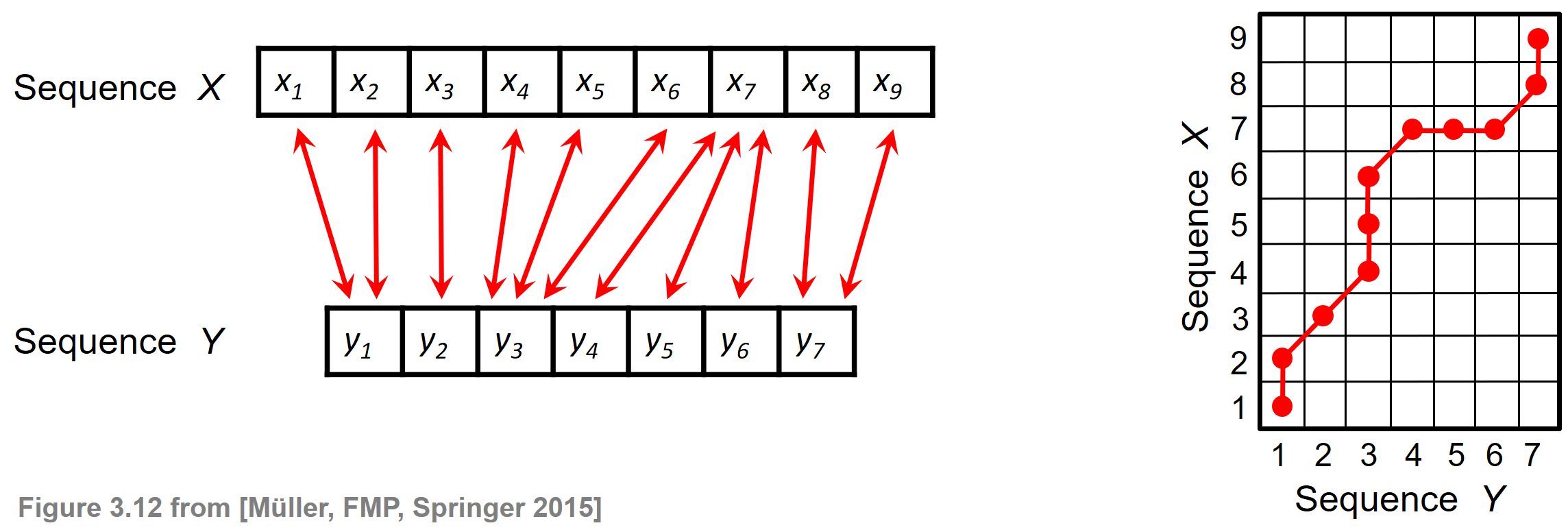

• 각각의 빨간색 양방향 화살표는 \(n\in[1:N]\) 및 \(m\in[1:M]\)에 대한 두 요소 \(x_n\) 및 \(y_m\) 간의 대응 관계를 인코딩한다. 이러한 로컬 대응은 인덱스 쌍 \((n,m)\)로 모델링할 수 있다. 위 그림의 오른쪽은 왼쪽에 표시된 정렬이 일련의 인덱스 쌍으로 인코딩되는 방식을 보여준다.

워핑 경로 (Warping Path)

• 시퀀스 \(X\) 및 \(Y\)의 원소 간 전역(global) 정렬을 모델링하려면, 특정 제약 조건을 충족하는 인덱스 쌍(pairs) 시퀀스를 고려하는 것이 좋다.

• 이것은 워핑 경로라는 개념으로 이어진다. 정의에 따르면 \(L\in\mathbb{N}\) 길이의 \((N,M)\)-워핑 경로는 다음의 시퀀스와 같다.

  • \(P=(p_1,\ldots,p_L)\)
  • with \(p_\ell=(n_\ell,m_\ell)\in[1:N]\times [1:M]\) for \(\ell\in[1:L]\)

• 그리고 다음의 세가지 조건을 만족한다.

  • 경계 조건(Boundary condition): \(p_1= (1,1)\) and \(p_L=(N,M)\)
  • 단조 조건(Monotonicity condition): \(n_1\leq n_2\leq\ldots \leq n_L\) and \(m_1\leq m_2\leq \ldots \leq m_L\)
  • 단계-크기 조건(Step-size condition): \(p_{\ell+1}-p_\ell\in \Sigma:=\{(1,0),(0,1),(1,1)\}\) for \(\ell\in[1:L]\)

• \((N,M)\)-워핑 경로 \(P=(p_1,\ldots,p_L)\)는 두 시퀀스 \(X=(x_1,x_2,\ldots,x_N)\) 및 \(Y=(y_1,y_2,\ldots,y_M)\) 사이의 정렬을 \(X\)의 원소 \(x_{n_\ell}\)를 \(Y\)의 원소 \(y_{m_\ell}\)에 할당하여 정의한다.

• 경계 조건(boundary condition)은 \(X\) 및 \(Y\)의 첫 번째 원소와 \(X\) 및 \(Y\)의 마지막 원소가 서로 정렬되도록 강제한다.

• 단조 조건(monotonicity condition)은 정확한 타이밍의 요구 사항을 반영한다. \(X\)의 원소가 \(X\)의 두 번째 원소 앞에 오는 경우 \(Y\)의 해당 원소에도 적용되어야 하며 그 반대의 경우도 마찬가지이다.

• 마지막으로 집합 \(\Sigma\)에 대한 단계-크기 조건(step-size condition)은 일종의 연속성 조건을 나타낸다. \(X\) 및 \(Y\)의 원소는 생략할 수 없으며 정렬에 복제가 없다.

• 다음 그림은 세 조건(boundary, monotonicity, step-size)이 위반되는 예를 각각 보여준다.

Image("../img/4.music_synchronization/FMP_C3_F13.png", width=600)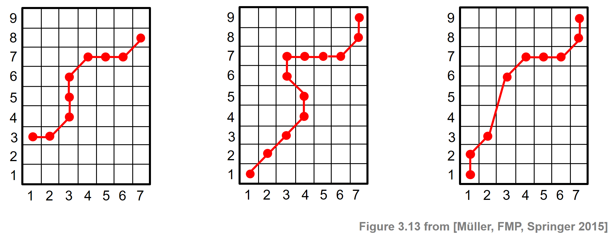

비용행렬과 최적성 (Cost Matrix and Optimality)

• 다음으로, 워핑 경로의 quality 에 대해 알려주는 개념을 살펴본다. 이를 위해서는 피쳐 시퀀스 \(X\)와 \(Y\)의 원소를 수치적으로 비교할 수 있는 방법이 필요하다. \(\mathcal{F}\)를 피쳐 공간으로 두고, \(x_n,y_m\in\mathcal{F}\) for \(n\in[1:N]\) and \(m\in[1:M]\)를 가정한다.

• 두 가지 다른 피쳐를 비교하려면 다음과 같은 함수로 정의된 로컬 비용 측정 (local cost measure)이 필요하다. \[c:\mathcal{F}\times\mathcal{F}\to \mathbb{R}\]

• 일반적으로 \(x\)와 \(y\)가 서로 유사하면 \(c(x,y)\)는 작고(저비용), 그렇지 않으면 \(c(x,y)\)가 크다(고비용). 시퀀스 \(X\) 및 \(Y\)의 각 원소 쌍에 대한 로컬 비용 측정값을 평가하면 다음과 같이 정의된 비용 매트릭스 (cost matirx) \(C\in\mathbb{R}^{N\times M}\)를 얻는다. \[C(n,m):=c(x_n,y_m)\] for \(n\in[1:N]\) and \(m\in[1:M]\).

• 행렬 \(C\)의 항목을 나타내는 튜플 \((n,m)\)은 행렬의 셀 (cell) 이라고 한다. 로컬 비용 측정 \(c\)와 관련하여 두 시퀀스 \(X\) 및 \(Y\) 사이의 워핑 경로 \(P\)의 총 비용 \(c_P(X,Y)\)는 다음과 같이 정의된다. \[ c_P:=\sum_{\ell=1}^L c(x_{n_\ell},y_{m_\ell}) = \sum_{\ell=1}^L C(n_\ell,m_\ell)\]

• 위 정의는 워핑 경로가 통과하는 모든 셀의 비용을 누적한다. 워핑 경로는 총 비용이 낮으면 “좋은 것”이고 총 비용이 높으면 “나쁜 것”이다.

• 이제 \(X\)와 \(Y\) 사이의 최적 워핑 경로 (optimal warping path) 를 보자. 이는 가능한 모든 워핑 경로 중에서 총 비용이 최소인 워핑 경로 \(P^\ast\)로 정의된다.

• 이 워핑 경로의 셀은 두 시퀀스의 원소 간의 전반적인 최적 정렬을 인코딩한다. 여기서 워핑 경로 조건은 \(X\) 시퀀스의 각 원소가 \(Y\)의 적어도 하나의 원소에 할당되며 그 반대의 경우도 마찬가지다.

• 이것은 길이 \(N\)의 \(X\)와 길이 \(M\)의 \(Y\) 사이에서 \(\mathrm{DTW}(X,Y)\)로 표시되는 DTW 거리(distance) 의 정의로 이어진다. 이는 최적의 \((N,M)\)-워핑 경로 \(P^\ast\)의 총 비용으로 정의된다. \[\mathrm{DTW}(X,Y) :=c_{P^\ast}(X,Y) = \min\{c_P(X,Y)\mid P \mbox{ is an $(N,M)$-warping path} \}\]

동적 프로그래밍(Dynamic Programming)을 이용한 DTW 알고리즘

• 두 시퀀스 \(X\) 및 \(Y\)에 대한 최적의 워핑 경로 \(P^\ast\)를 결정하기 위해 가능한 모든 \((N,M)\) 워핑 경로의 총 비용을 계산한 다음 최소 비용을 취할 수 있다. 그러나 다른 \((N,M)\) 워핑 경로의 수는 \(N\) 및 \(M\)에서 기하급수적이다. 따라서 이러한 접근 방식은 큰 \(N\) 및 \(M\)에 대해 계산적으로 실행 불가능하다.
• 동적 프로그래밍 (Dynamic Programming) 에 기반한 \(O(NM)\) 알고리즘을 보자. 동적 프로그래밍의 주요 아이디어는 주어진 문제를 더 간단한 하위 문제로 분해한 다음 하위 문제의 솔루션을 결합하여 전체 솔루션에 도달하는 것이다.
• DTW의 경우 잘린 하위 시퀀스에 대한 최적 워핑 경로에서 원본 시퀀스에 대한 최적 워핑 경로를 도출하는 것이 방법이다. 그런 다음 이 방법을 재귀적으로 적용할 수 있다. 이를 공식화하기 위해 prefix 시퀀스를 정의한다.
  • \(X(1\!:\!n) := (x_1,\ldots x_n)\) for \(n\in[1:N]\)
  • \(Y(1\!:\!m) := (y_1,\ldots y_m)\) for \(m\in[1:M]\)
  • and set \(D(n,m):=\mathrm{DTW}(X(1\!:\!n),Y(1\!:\!m))\)
• \(D\) 값은 누적 비용 행렬(accumulated cost matrix) 이라고도 하는 \((N\times M)\) 행렬 \(D\)를 정의한다. 각 값 \(D(n,m)\)은 셀 \((1,1)\)에서 시작하여 셀 \((n,m)\)에서 끝나는 최적 워핑 경로의 총(또는 누적) 비용을 지정한다. \(D(N,M)=\mathrm{DTW}(X,Y)\)는 반드시 있다.
• 다음 표는 동적 프로그래밍에 기반한 DTW 알고리즘에 대한 설명이다.
  • 첫 번째 부분에서 누적 비용 행렬 \(D\)는 중첩 루프를 사용하여 반복적으로 계산된다.
  • 두 번째 부분에서는 역추적 절차를 사용하여 최적의 워핑 경로를 계산한다.

Image("../img/4.music_synchronization/FMP_C3_T02.png", width=600)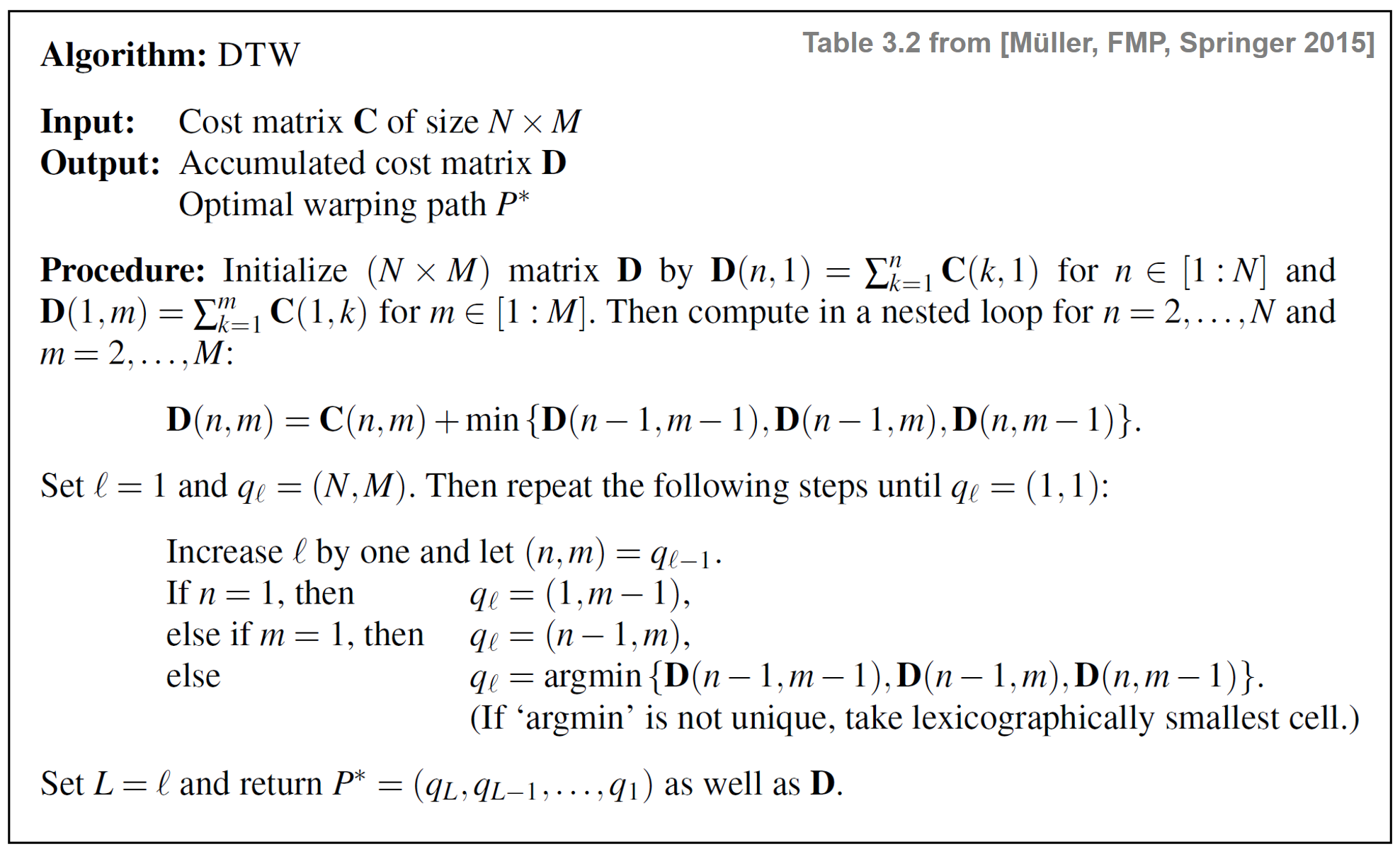

예시

# 길이가 다른 두 시퀀스
X =  [1, 3, 9, 2, 1] #시퀀스
Y = [2, 0, 0, 8, 7, 2] #시퀀스
N = len(X)
M = len(Y)

plt.figure(figsize=(6, 2))
plt.plot(X, c='k', label='$X$')
plt.plot(Y, c='b', label='$Y$')
plt.legend()
plt.tight_layout()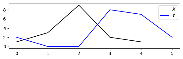

def compute_cost_matrix(X, Y, metric='euclidean'):
    """Compute the cost matrix of two feature sequences

    Args:
        X (np.ndarray): Sequence 1
        Y (np.ndarray): Sequence 2
        metric (str): Cost metric, a valid strings for scipy.spatial.distance.cdist (Default value = 'euclidean')

    Returns:
        C (np.ndarray): Cost matrix
    """
    X, Y = np.atleast_2d(X, Y)
    C = scipy.spatial.distance.cdist(X.T, Y.T, metric=metric)
    return C

# 비용행렬 계산
C =  compute_cost_matrix(X, Y, metric='euclidean')
print('Cost matrix C =', C, sep='\n')

Cost matrix C =
[[1. 1. 1. 7. 6. 1.]
 [1. 3. 3. 5. 4. 1.]
 [7. 9. 9. 1. 2. 7.]
 [0. 2. 2. 6. 5. 0.]
 [1. 1. 1. 7. 6. 1.]]

def compute_accumulated_cost_matrix(C):
    """Compute the accumulated cost matrix given the cost matrix

    Args:
        C (np.ndarray): Cost matrix

    Returns:
        D (np.ndarray): Accumulated cost matrix
    """
    N = C.shape[0]
    M = C.shape[1]
    D = np.zeros((N, M))
    D[0, 0] = C[0, 0]
    for n in range(1, N):
        D[n, 0] = D[n-1, 0] + C[n, 0]
    for m in range(1, M):
        D[0, m] = D[0, m-1] + C[0, m]
    for n in range(1, N):
        for m in range(1, M):
            D[n, m] = C[n, m] + min(D[n-1, m], D[n, m-1], D[n-1, m-1])
    return D

# 누적 비용행렬 계산
D =  compute_accumulated_cost_matrix(C)
print('Accumulated cost matrix D =', D, sep='\n')
print('DTW distance DTW(X, Y) =', D[-1, -1])

Accumulated cost matrix D =
[[ 1.  2.  3. 10. 16. 17.]
 [ 2.  4.  5.  8. 12. 13.]
 [ 9. 11. 13.  6.  8. 15.]
 [ 9. 11. 13. 12. 11.  8.]
 [10. 10. 11. 18. 17.  9.]]
DTW distance DTW(X, Y) = 9.0

def compute_optimal_warping_path(D):
    """Compute the warping path given an accumulated cost matrix

    Args:
        D (np.ndarray): Accumulated cost matrix

    Returns:
        P (np.ndarray): Optimal warping path
    """
    N = D.shape[0]
    M = D.shape[1]
    n = N - 1
    m = M - 1
    P = [(n, m)]
    while n > 0 or m > 0:
        if n == 0:
            cell = (0, m - 1)
        elif m == 0:
            cell = (n - 1, 0)
        else:
            val = min(D[n-1, m-1], D[n-1, m], D[n, m-1])
            if val == D[n-1, m-1]:
                cell = (n-1, m-1)
            elif val == D[n-1, m]:
                cell = (n-1, m)
            else:
                cell = (n, m-1)
        P.append(cell)
        (n, m) = cell
    P.reverse()
    return np.array(P)

# 최적 warping path 계산
P = compute_optimal_warping_path(D)
print('Optimal warping path P =', P.tolist())

Optimal warping path P = [[0, 0], [0, 1], [1, 2], [2, 3], [2, 4], [3, 5], [4, 5]]

c_P = sum(C[n, m] for (n, m) in P)
print('Total cost of optimal warping path:', c_P)
print('DTW distance DTW(X, Y) =', D[-1, -1])

Total cost of optimal warping path: 9.0
DTW distance DTW(X, Y) = 9.0

P = np.array(P) 
plt.figure(figsize=(8, 3))
plt.subplot(1, 2, 1)
plt.imshow(C, cmap='gray_r', origin='lower', aspect='equal')
plt.plot(P[:, 1], P[:, 0], marker='o', color='r')
plt.clim([0, np.max(C)])
plt.colorbar()
plt.title('$C$ with optimal warping path')
plt.xlabel('Sequence Y')
plt.ylabel('Sequence X')

plt.subplot(1, 2, 2)
plt.imshow(D, cmap='gray_r', origin='lower', aspect='equal')
plt.plot(P[:, 1], P[:, 0], marker='o', color='r')
plt.clim([0, np.max(D)])
plt.colorbar()
plt.title('$D$ with optimal warping path')
plt.xlabel('Sequence Y')
plt.ylabel('Sequence X')

plt.tight_layout()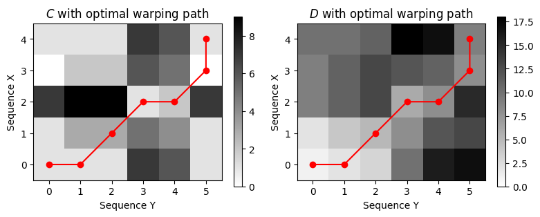

## librosa example

D, P = librosa.sequence.dtw(X, Y, metric='euclidean', 
                            step_sizes_sigma=np.array([[1, 1], [0, 1], [1, 0]]),
                            weights_add=np.array([0, 0, 0]), weights_mul=np.array([1, 1, 1]))

plt.figure(figsize=(8, 3))
ax = plt.subplot(1,1,1)
plot_matrix_with_points(D, P, linestyle='-', 
    ax=[ax], aspect='equal', clim=[0, np.max(D)],
    title='$D$ with optimal warping path', xlabel='Sequence Y', ylabel='Sequence X');

plt.tight_layout()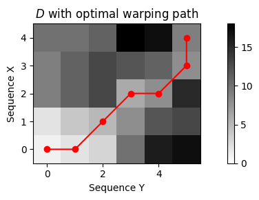

DTW 변형

단계 크기 조건 (Step-size Condition)

• 기존 DTW에서 step-size 조건은 \(\Sigma=\{(1,0),(0,1),(1,1)\}\) 집합으로 표현된다. 일종의 local 연속성 조건을 도입하는 이 조건은 워핑 경로가 시퀀스 \(X=(x_1,x_2,\ldots,x_N)\)의 각 원소를 \(Y=(y_1,y_2,\ldots, y_M)\)의 원소로 할당하도록 하며 그 반대도 마찬가지이다.
• 이 조건의 한 가지 단점은 한 시퀀스의 단일 원소가 다른 시퀀스의 많은 연속된 원소에 할당되어 워핑 경로에서 수직 및 수평 섹션으로 이어질 수 있다는 것이다.
• 직관적으로 이러한 경우 워핑 경로는 시퀀스 중 하나의 시퀀스에서는 특정 위치에 고정되고 다른 시퀀스에서는 이동한다. 물리적 시간 측면에서 이 상황은 두 시계열의 정렬에서 강한 시간적 변형(temporal deformation)에 해당된다. 이러한 변성을 피하기 위해 허용 가능한 워핑 경로의 기울기를 제한하여 step-size 조건을 수정할 수 있다.
• 이는 집합 \(\Sigma\)를 교체하여 수행할 수 있다.

Image("../img/4.music_synchronization/FMP_C3_F17.png", width=600)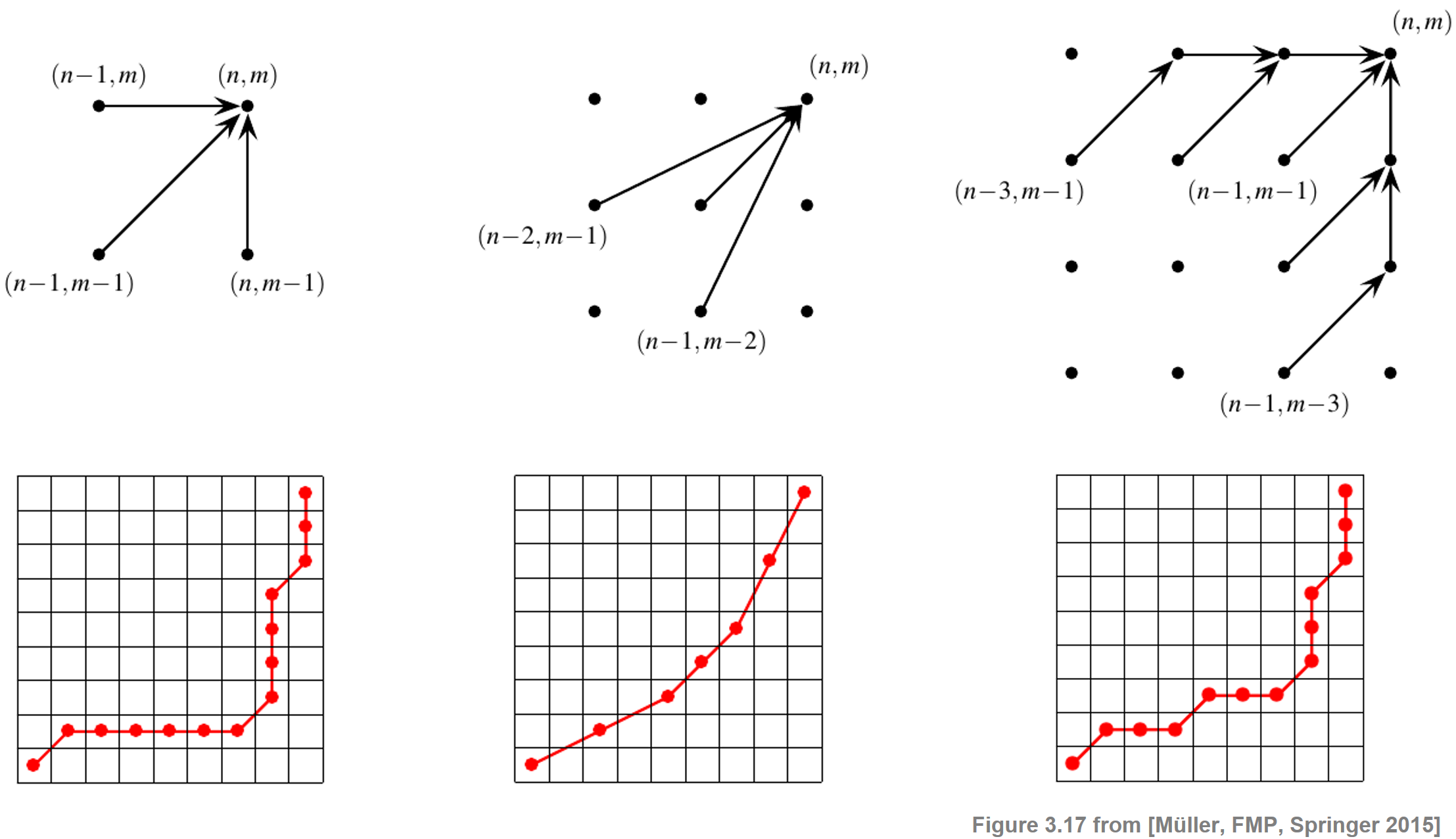

• 첫 번째 경우 원래의 집합 \(\Sigma=\{(1,0),(0,1),(1,1)\}\)가 사용된다(워핑 경로의 degeneration 관찰).

• 이 집합을 \(\Sigma = \{(2,1),(1,2),(1,1)\}\)과 같이 교체하면 워핑 경로가 \(1/2\) 및 \(2\) 범위 내에서 local 기울기를 갖는 워핑 경로로 이어진다.

• 새로운 step size 제약을 만족하는 최적 워핑 경로를 계산하기 위해 원래의 DTW 알고리즘을 조금만 변형하면 된다. 누적 비용행렬 \(\mathbf{D}\)을 계산하기 위해 다음의 recursion을 사용한다. \[\mathbf{D}(n,m)= \mathbf{C}(n,m) + \min\left\{ \begin{array}{l}\mathbf{D}(n-1,m-1),\\ \mathbf{D}(n-2,m-1),\\\mathbf{D}(n-1,m-2) \end{array}\right.\] for \(n\in [1:N]\) and \(m\in [1:N]\) with \((n,m)\not=(1,1)\).

• 초기화를 위해 \(\mathbf{D}\)를 두 개의 추가 행과 열(\(-1\) 및 \(0\)로 인덱싱됨), 그리고 집합 \(\mathbf{D}(1,1):=\mathbf{C}(1,1)\), \(\mathbf{D}(n,-1):=\mathbf{D}(n,0):=\infty\) for \(n\in [-1:N]\)와 \(\mathbf{D}(-1,m):=\mathbf{D}(0,m):=\infty\) for \(m\in [-1:M]\) 로 확장하는 트릭을 사용할 수 있다.

• 수정된 step-size 조건과 관련하여 두 시퀀스 \(X\)와 \(Y\) 사이에 유한의 총 비용 워핑 경로가 있다. 또한 \(X\)의 모든 원소를 \(Y\)의 일부 원소에 할당할 필요는 없으며 그 반대도 마찬가지다(위 그림 참조). 위 그림의 세 번째 경우는 워핑 경로의 기울기에 제약을 가하면서 이러한 누락을 피하는 step-size 조건을 보여준다.

def compute_accumulated_cost_matrix_21(C):
    """Compute the accumulated cost matrix given the cost matrix

    Args:
        C (np.ndarray): Cost matrix

    Returns:
        D (np.ndarray): Accumulated cost matrix
    """
    N = C.shape[0]
    M = C.shape[1]
    D = np.zeros((N + 2, M + 2))
    D[:, 0:2] = np.inf
    D[0:2, :] = np.inf
    D[2, 2] = C[0, 0]

    for n in range(N):
        for m in range(M):
            if n == 0 and m == 0:
                continue
            D[n+2, m+2] = C[n, m] + min(D[n-1+2, m-1+2], D[n-2+2, m-1+2], D[n-1+2, m-2+2])
    D = D[2:, 2:]
    return D


def compute_optimal_warping_path_21(D):
    """Compute the warping path given an accumulated cost matrix

    Args:
        D (np.ndarray): Accumulated cost matrix

    Returns:
        P (np.ndarray): Optimal warping path
    """
    N = D.shape[0]
    M = D.shape[1]
    n = N - 1
    m = M - 1
    P = [(n, m)]
    while n > 0 or m > 0:
        if n == 0:
            cell = (0, m - 1)
        elif m == 0:
            cell = (n - 1, 0)
        else:
            val = min(D[n-1, m-1], D[n-2, m-1], D[n-1, m-2])
            if val == D[n-1, m-1]:
                cell = (n-1, m-1)
            elif val == D[n-2, m-1]:
                cell = (n-2, m-1)
            else:
                cell = (n-1, m-2)
        P.append(cell)
        (n, m) = cell
    P.reverse()
    P = np.array(P)
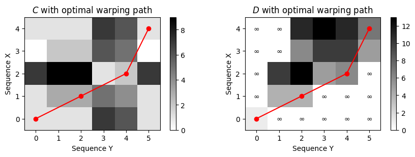
    return P

# Sequences
X = [1, 3, 9, 2, 1]
Y = [2, 0, 0, 8, 7, 2]
N, M = len(X), len(Y)

C = compute_cost_matrix(X, Y, metric='euclidean')
D = compute_accumulated_cost_matrix_21(C)
P = compute_optimal_warping_path_21(D)  
    
plt.figure(figsize=(6, 2))
plt.plot(X, c='k', label='X')
plt.plot(Y, c='b', label='Y')
plt.legend()
plt.tight_layout()

plt.figure(figsize=(9, 3))
ax = plt.subplot(1, 2, 1)
plot_matrix_with_points(C, P, linestyle='-', 
    ax=[ax], aspect='equal', clim=[0, np.max(C)],
    title='$C$ with optimal warping path', xlabel='Sequence Y', ylabel='Sequence X');

ax = plt.subplot(1, 2, 2)
D_max = np.nanmax(D[D != np.inf])
plot_matrix_with_points(D, P, linestyle='-', 
    ax=[ax], aspect='equal', clim=[0, D_max],
    title='$D$ with optimal warping path', xlabel='Sequence Y', ylabel='Sequence X');
for x, y in zip(*np.where(np.isinf(D))):
    plt.text(y, x, '$\infty$', horizontalalignment='center', verticalalignment='center')

plt.tight_layout()

## librosa 예

def compute_plot_D_P(X, Y, ax, step_sizes_sigma=np.array([[1, 1], [0, 1], [1, 0]]),
                     weights_mul=np.array([1, 1, 1]), title='',
                     global_constraints=False, band_rad=0.25):
    D, P = librosa.sequence.dtw(X, Y, metric='euclidean', weights_mul=weights_mul,
                    step_sizes_sigma=step_sizes_sigma, 
                    global_constraints=global_constraints, band_rad=band_rad)
    D_max = np.nanmax(D[D != np.inf])
    plot_matrix_with_points(D, P, linestyle='-', 
        ax=[ax], aspect='equal', clim=[0, D_max],
        title= title, xlabel='Sequence Y', ylabel='Sequence X');
    for x, y in zip(*np.where(np.isinf(D))):
        plt.text(y, x, '$\infty$', horizontalalignment='center', verticalalignment='center')
    
X = [1, 3, 9, 2, 1, 3, 9, 9]
Y = [2, 0, 0, 9, 1, 7]  

print('다양한 step-size 조건에 대한 누적 비용 행렬 및 최적 워핑 경로:')
plt.figure(figsize=(10, 3))

ax = plt.subplot(1, 3, 1)
step_sizes_sigma = np.array([[1, 0], [0, 1], [1, 1]])
title='Step sizes:'+''.join(str(s) for s in step_sizes_sigma)
compute_plot_D_P(X, Y, ax=ax, step_sizes_sigma=step_sizes_sigma, title=title)

ax = plt.subplot(1, 3, 2)
step_sizes_sigma = np.array([[1, 1], [2, 1], [1, 2]])
title='Step sizes:'+''.join(str(s) for s in step_sizes_sigma)
compute_plot_D_P(X, Y, ax=ax, step_sizes_sigma=step_sizes_sigma, title=title)

ax = plt.subplot(1, 3, 3)
step_sizes_sigma = np.array([[1, 1], [3, 1], [1, 3]])
title='Step sizes:'+''.join(str(s) for s in step_sizes_sigma)                                                       
compute_plot_D_P(X, Y, ax=ax, step_sizes_sigma=step_sizes_sigma, title=title)

plt.tight_layout()

다양한 step-size 조건에 대한 누적 비용 행렬 및 최적 워핑 경로: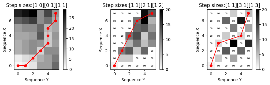

로컬 가중치 (Local Weights)

• 정렬에 수직, 수평 또는 대각선 방향 등 특정 방향을 선호한다면, 추가 로컬 가중치 (local weights) \(w_{\mathrm{d}},w_{\mathrm{h}},w_{\mathrm{v}}\in\mathbb{R}\)를 도입할 수 있다. 누적 비용 행렬 \(\mathbf{D}\)를 계산하기 위해 다음 initialization 및 recursion을 사용한다.

\[\mathbf{D}(1,1):=\mathbf{C}(1,1)\] \[\mathbf{D}(n,1)=\sum_{k=1}^{n} w_{\mathrm{h}}\cdot \mathbf{C}(k,1) \,\,\mbox{for}\,\, n\in [2:N]\] \[\mathbf{D}(1,m)=\sum_{k=1}^{m} w_{\mathrm{v}}\cdot \mathbf{C}(1,k) \,\,\mbox{for}\,\, m\in [2:M]\] \[\mathbf{D}(n,m)=\min \left\{ \begin{array}{l} \mathbf{D}(n-1,m-1) + w_{\mathrm{d}}\cdot \mathbf{C}(n,m) \\ \mathbf{D}(n-1,m) + w_{\mathrm{v}}\cdot \mathbf{C}(n,m) \\ \mathbf{D}(n,m-1) + w_{\mathrm{h}}\cdot \mathbf{C}(n,m) \end{array} \right.\]

for \(n\in[2:N]\) and \(m\in[2:M]\).

• \(w_{\mathrm{d}}=w_{\mathrm{h}}=w_{\mathrm{v}}=1\)이면 기존 DTW로 축소된다.
• 기본적으로 하나의 대각선 단계(셀 하나의 비용)가 하나의 수평 단계와 하나의 수직 단계(두 셀의 비용)의 조합에 해당하기 때문에, 대각선 정렬 방향을 선호한다. 이러한 선호의 균형을 맞추기 위해 종종 \(w_{\mathrm{d}}=2\) 및 \(w_{\mathrm{h}}=w_{\mathrm{v}}=1\)를 선택한다.
• 마찬가지로 다른 step-size 조건에 대한 가중치를 도입할 수 있다.
• 다음 코드 셀에서 다른 가중치 설정으로 librosa.sequence.dtw 함수를 호출한다.

X = [1, 1, 1, 1, 2, 1, 1, 6, 6]
Y = [0, 3, 3, 3, 9, 9, 7, 7]

print(r'다양한 local 가중치에 따른 누적 비용 행렬과 최적 warping 경로:')
plt.figure(figsize=(10, 3))

ax = plt.subplot(1, 3, 1)
weights_mul = np.array([1, 1, 1])
title='Weights: '+'[ '+''.join(str(s)+' ' for s in weights_mul)+']'
compute_plot_D_P(X, Y, ax=ax, weights_mul=weights_mul, title=title)

ax = plt.subplot(1, 3, 2)
weights_mul = np.array([2, 1, 1])
title='Weights: '+'[ '+''.join(str(s)+' ' for s in weights_mul)+']'
compute_plot_D_P(X, Y, ax=ax, weights_mul=weights_mul, title=title)

ax = plt.subplot(1, 3, 3)
weights_mul = np.array([1, 3, 3])
title='Weights: '+'[ '+''.join(str(s)+' ' for s in weights_mul)+']'                                                      
compute_plot_D_P(X, Y, ax=ax, weights_mul=weights_mul, title=title)

plt.tight_layout()

다양한 local 가중치에 따른 누적 비용 행렬과 최적 warping 경로: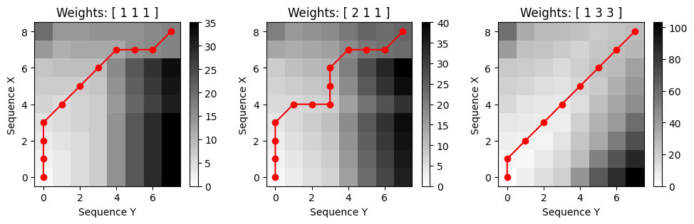

전역 제약 (Global Constraints)

• 일반적인 DTW 변형 중 하나는 허용 가능한 워핑 경로에 전역 제약(global constraint)을 부과하는 것이다.

• 이러한 제약 조건은 DTW 계산 속도를 높일 뿐만 아니라 워핑 경로의 전체 과정을 전체적으로 제어하여 “pathological” 정렬을 방지한다.

• 보다 정확하게는 \(R\subseteq [1:N]\times[1:M]\)를 전역적 제약 영역이라고 하는 하위 집합이라고 하자. 그러면 \(R\)과 연관된(relative to) 워핑 경로 는 \(R\) 지역 내에서 완전히 실행되는 워핑 경로이다.

• \(P^\ast_{R}\)로 표시되는 \(R\)과 연관된 최적 워핑 경로 는 \(R\)에 대한 모든 워핑 경로 중에서 비용을 최소화하는 워핑 경로이다.

• 다음 그림은 Sakoe–Chiba 밴드 및 Itakura 평행사변형으로 알려진 두 개의 전역 제약 영역을 보여준다. 셀의 정렬은 각 음영 영역에서만 선택할 수 있다.

Image("../img/4.music_synchronization/FMP_C3_F18_text.png", width=600)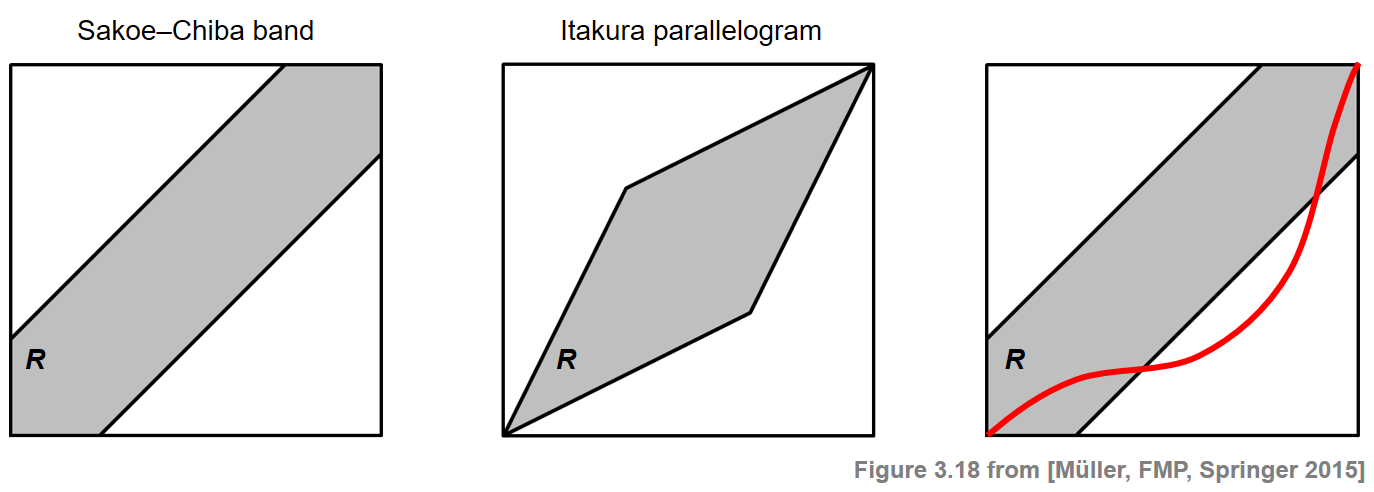

• 일반적으로 제약 영역 \(R\)의 경우, 경로 \(P^\ast_{R}\)는 \(\mathbf{C}(n,m):=\infty\) for all \((n,m)\in [1:N]\times[1:M]\setminus R\)로 세팅하여 제약 없는 경우와 유사하게 계산할 수 있다.

• 따라서 \(P^\ast_{R}\) 계산에서 \(R\)에 있는 셀만 평가하면 된다. 이렇게 하면 DTW 계산 속도가 상당히 빨라질 수 있다. 그러나 제약되지 않은 최적 워핑 경로 \(P^\ast\)가 지정된 제약 영역 외부의 셀을 통과할 수 있기 때문에 전역 제약 영역의 사용 또한 문제가 된다. 이 경우 제한된 최적 워핑 경로 \(P^\ast_{R}\)는 \(P^\ast\)와 일치하지 않는다(위 그림의 마지막 경우 참조).

• 다음 코드 셀에서 Sakoe-Chiba 밴드에 의해 결정된 다양한 제약 영역으로 librosa.sequence.dtw 함수를 사용해본다.

• 다음의 예에서 워핑 경로는 \((1, 1)\)에서 시작하지 않는데, 이는 librosa의 역추적 버그 때문이다.(차후 수정될 수 있음)

X = [1, 1, 1, 1, 2, 1, 1, 6, 6]
Y = [0, 3, 3, 3, 9, 9, 7, 7]

print(r'Accumulated cost matrix and optimal warping path for different constraint regions:')
plt.figure(figsize=(10, 3))
global_constraints = True

ax = plt.subplot(1, 3, 1)
band_rad = 1
title='Sakao-Chiba band (rad = %.2f)'%band_rad
compute_plot_D_P(X, Y, ax=ax, global_constraints=global_constraints, band_rad=band_rad,title=title)

ax = plt.subplot(1, 3, 2)
band_rad = 0.5
title='Sakao-Chiba band (rad = %.2f)'%band_rad
compute_plot_D_P(X, Y, ax=ax, global_constraints=global_constraints, band_rad=band_rad,title=title)

ax = plt.subplot(1, 3, 3)
band_rad = 0.25
title='Sakao-Chiba band (rad = %.2f)'%band_rad
compute_plot_D_P(X, Y, ax=ax, global_constraints=global_constraints, band_rad=band_rad,title=title)

plt.tight_layout()

Accumulated cost matrix and optimal warping path for different constraint regions: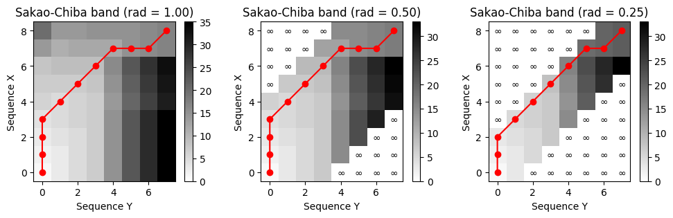

멀티스케일 (Multiscale) DTW

• global 제약 영역의 개념을 사용할 때, 계산할 최적 워핑 경로가 실제로 이 영역 내에 있는지 확인해야 한다. 이 경로는 선험적으로 알려져 있지 않기 때문에, 제한 영역을 가능한 한 작게 선택(계산 속도를 높이기 위해)하지만 원하는 경로를 포함할 만큼 충분히 크게 선택하는 것 사이에서 적절한 절충점을 찾기가 어렵다.
• “올바른” 경로를 찾을 확률을 높이는 한 가지 가능한 전략은 데이터 독립적인 고정 제약 조건 영역 대신 데이터 종속 제약 조건 영역을 사용하는 것이다. 이 아이디어는 DTW에 대한 멀티스케일 접근 방식 (multiscale approach) 에 의해 실현될 수 있다.
• 여기서 일반적인 전략은 재귀적으로 거친 해상도 수준에서 계산된 최적 워핑 경로를 다음 상위 수준으로 투영한 다음, 투영된 경로를 미세 조정하는 것이다. 다음 그림은 이러한 접근 방식의 주요 단계를 요약한 것이다. 거친 해상도 수준에서 계산된 최적 워핑은 더 미세한 해상도 수준으로 투영된다. 작은 이웃과 함께(전체 절차의 견고성을 높이기 위해) 더 미세한 해상도 수준에서 워핑 경로를 계산하는 데 사용되는 제약 조건 영역을 정의한다.

Image("../img/4.music_synchronization/FMP_C3_F19.png", width=600)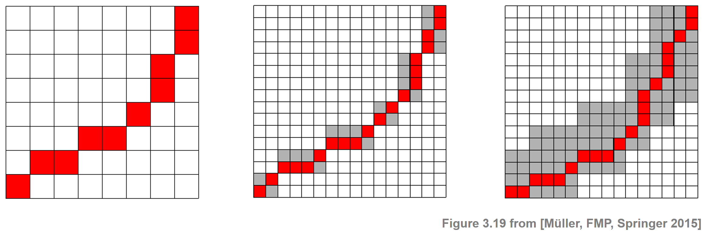

DTW 예시

• Librosa를 활용
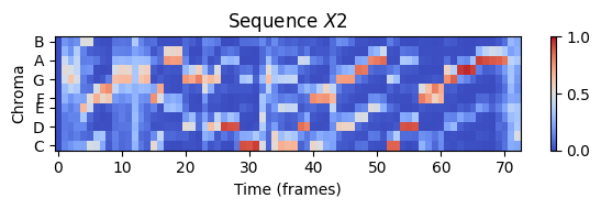
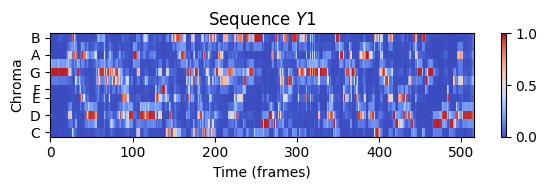
• 같은 노래(sir duke)의 느리고 빠른 버전, 같은 노래(bach goldberg)의 다른 연도 연주 버전을 비교하는 DTW를 보자.

# for mp3 files
import audioread.ffdec
mp3 = audioread.ffdec.FFmpegAudioFile('../audio/sir_duke_trumpet_fast.mp3')
x1, sr1 = librosa.load(mp3)
mp3 = audioread.ffdec.FFmpegAudioFile('../audio/sir_duke_trumpet_slow.mp3')
x2, sr2 = librosa.load(mp3)

x3, sr3 = librosa.load('../audio/gould_bach_goldberg_1955.wav')
x4, sr4 = librosa.load('../audio/gould_bach_goldberg_1981.wav')

N = 4410
H = 2205
X1 = librosa.feature.chroma_stft(y=x1, sr=sr1, tuning=0, norm=2, hop_length=H, n_fft=N)
X2 = librosa.feature.chroma_stft(y=x2, sr=sr2, tuning=0, norm=2, hop_length=H, n_fft=N)
Y1 = librosa.feature.chroma_stft(y=x3, sr=sr3, tuning=0, norm=2, hop_length=H, n_fft=N)
Y2 = librosa.feature.chroma_stft(y=x4, sr=sr4, tuning=0, norm=2, hop_length=H, n_fft=N)

plt.figure(figsize=(6, 2))
plt.title('Sequence $X1$')
librosa.display.specshow(X1, x_axis='frames', y_axis='chroma', cmap='coolwarm', hop_length=H)
plt.xlabel('Time (frames)')
plt.ylabel('Chroma')
plt.colorbar()
plt.clim([0, 1])
plt.tight_layout(); plt.show()
ipd.display(ipd.Audio(x1, rate=sr1))

plt.figure(figsize=(6, 2))
plt.title('Sequence $X2$')
librosa.display.specshow(X2, x_axis='frames', y_axis='chroma', cmap='coolwarm', hop_length=H)
plt.xlabel('Time (frames)')
plt.ylabel('Chroma')
plt.colorbar()
plt.clim([0, 1])
plt.tight_layout(); plt.show()
ipd.display(ipd.Audio(x2, rate=sr2))

plt.figure(figsize=(6, 2))
plt.title('Sequence $Y1$')
librosa.display.specshow(Y1, x_axis='frames', y_axis='chroma', cmap='coolwarm', hop_length=H)
plt.xlabel('Time (frames)')
plt.ylabel('Chroma')
plt.colorbar()
plt.clim([0, 1])
plt.tight_layout(); plt.show()
ipd.display(ipd.Audio(x3, rate=sr3))

plt.figure(figsize=(6, 2))
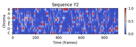
plt.title('Sequence $Y2$')
librosa.display.specshow(Y2, x_axis='frames', y_axis='chroma', cmap='coolwarm', hop_length=H)
plt.xlabel('Time (frames)')
plt.ylabel('Chroma')
plt.colorbar()
plt.clim([0, 1])
plt.tight_layout(); plt.show()
ipd.display(ipd.Audio(x4, rate=sr4))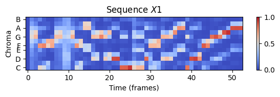

C = compute_cost_matrix(X1, X2)
D = compute_accumulated_cost_matrix(C)
P = compute_optimal_warping_path(D)


plt.figure(figsize=(10, 3))
ax = plt.subplot(1, 2, 1)
plot_matrix_with_points(C, P, linestyle='-',  marker='', 
    ax=[ax], aspect='equal', clim=[0, np.max(C)], 
    title='$C$ with optimal warping path', xlabel='Sequence X2', ylabel='Sequence X1');

ax = plt.subplot(1, 2, 2)
plot_matrix_with_points(D, P, linestyle='-', marker='', 
    ax=[ax], aspect='equal', clim=[0, np.max(D)], 
    title='$D$ with optimal warping path', xlabel='Sequence X2', ylabel='Sequence X1');

plt.tight_layout()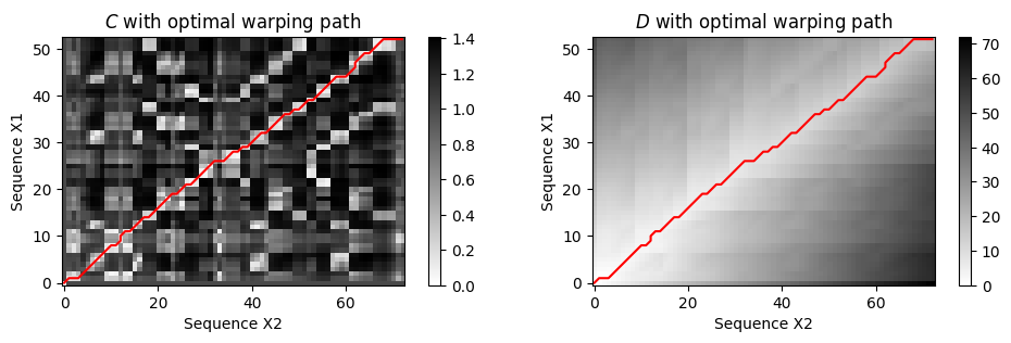

C2 = compute_cost_matrix(Y1, Y2)
D2 = compute_accumulated_cost_matrix(C2)
P2 = compute_optimal_warping_path(D2)


plt.figure(figsize=(10, 3))
ax = plt.subplot(1, 2, 1)
plot_matrix_with_points(C2, P2, linestyle='-',  marker='', 
    ax=[ax], aspect='equal', clim=[0, np.max(C2)], 
    title='$C$ with optimal warping path', xlabel='Sequence Y2', ylabel='Sequence Y1');

ax = plt.subplot(1, 2, 2)
plot_matrix_with_points(D2, P2, linestyle='-', marker='', 
    ax=[ax], aspect='equal', clim=[0, np.max(D2)], 
    title='$D$ with optimal warping path', xlabel='Sequence Y2', ylabel='Sequence Y1');

plt.tight_layout()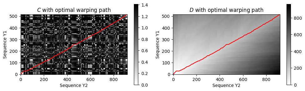

N = X1.shape[1]
M = X2.shape[1]

plt.figure(figsize=(8, 3))
#plt.figure(figsize=(5, 3)) 
ax_X = plt.axes([0, 0.60, 1, 0.40])
librosa.display.specshow(X1, ax=ax_X, x_axis='frames', y_axis='chroma', cmap='coolwarm', hop_length=H)
ax_X.set_ylabel('Sequence X1')
ax_X.set_xlabel('Time (frames)')
ax_X.xaxis.tick_top()
ax_X.xaxis.set_label_position('top') 

ax_Y = plt.axes([0, 0, 1, 0.40])
librosa.display.specshow(X2, ax=ax_Y, x_axis='frames', y_axis='chroma', cmap='coolwarm', hop_length=H)
ax_Y.set_ylabel('Sequence X2')
ax_Y.set_xlabel('Time (frames)')

step = 5
y_min_X, y_max_X = ax_X.get_ylim()
y_min_Y, y_max_Y = ax_Y.get_ylim()
for t in P[0:-1:step, :]: 
    ax_X.vlines(t[0], y_min_X, y_max_X, color='r')
    ax_Y.vlines(t[1], y_min_Y, y_max_Y, color='r')

ax = plt.axes([0, 0.40, 1, 0.20])
for p in P[0:-1:step, :]: 
    ax.plot((p[0]/N, p[1]/M), (1, -1), color='r')
    ax.set_xlim(0, 1)
    ax.set_ylim(-1, 1)
ax.set_xticks([])
ax.set_yticks([]);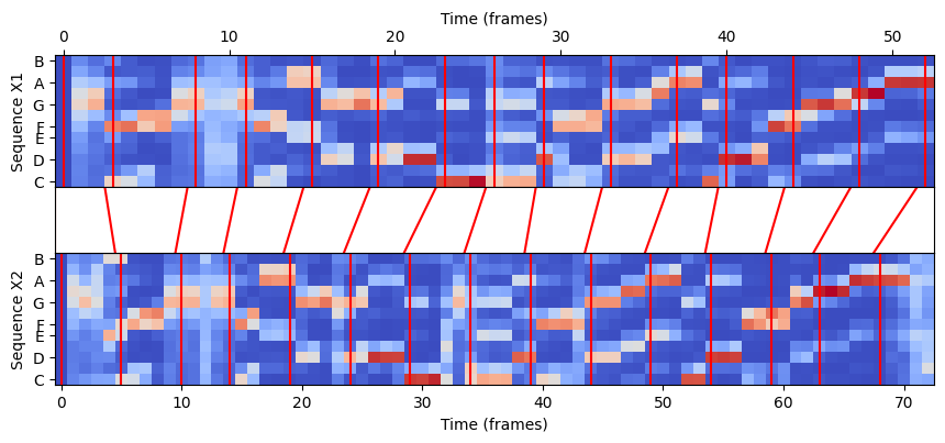

N = Y1.shape[1]
M = Y2.shape[1]

plt.figure(figsize=(8, 3))
#plt.figure(figsize=(5, 3)) 
ax_X = plt.axes([0, 0.60, 1, 0.40])
librosa.display.specshow(Y1, ax=ax_X, x_axis='frames', y_axis='chroma', cmap='coolwarm', hop_length=H)
ax_X.set_ylabel('Sequence Y1')
ax_X.set_xlabel('Time (frames)')
ax_X.xaxis.tick_top()
ax_X.xaxis.set_label_position('top') 

ax_Y = plt.axes([0, 0, 1, 0.40])
librosa.display.specshow(Y2, ax=ax_Y, x_axis='frames', y_axis='chroma', cmap='coolwarm', hop_length=H)
ax_Y.set_ylabel('Sequence Y2')
ax_Y.set_xlabel('Time (frames)')

step = 30
y_min_X, y_max_X = ax_X.get_ylim()
y_min_Y, y_max_Y = ax_Y.get_ylim()
for t in P2[0:-1:step, :]: 
    ax_X.vlines(t[0], y_min_X, y_max_X, color='r')
    ax_Y.vlines(t[1], y_min_Y, y_max_Y, color='r')

ax = plt.axes([0, 0.40, 1, 0.20])
for p in P2[0:-1:step, :]: 
    ax.plot((p[0]/N, p[1]/M), (1, -1), color='r')
    ax.set_xlim(0, 1)
    ax.set_ylim(-1, 1)
ax.set_xticks([])
ax.set_yticks([]);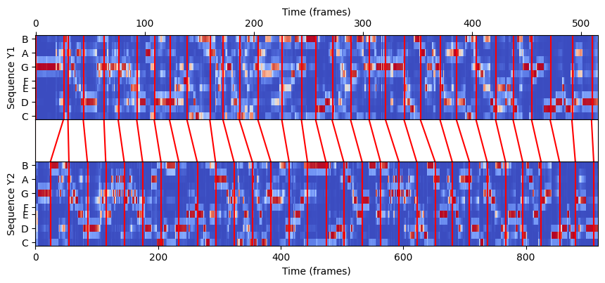

---

출처:

• https://www.audiolabs-erlangen.de/resources/MIR/FMP/C3/C3S2_DTWbasic.html
• https://www.audiolabs-erlangen.de/resources/MIR/FMP/C3/C3S2_DTWvariants.html
• https://www.audiolabs-erlangen.de/resources/MIR/FMP/C3/C3_MusicSynchronization.html
• https://musicinformationretrieval.com/

---

구글 Colab 링크

---

\(\leftarrow\) 4.1. 오디오 동기화 피쳐

5.1. 음악 구조와 분할 \(\rightarrow\)